Ontem, a FGV divulgou o seu Índice de Incerteza Econômica Brasil. Como esperado, houve um aumento em agosto. Com efeito, a incerteza permanece acima da média histórica. Para ilustrar, podemos usar o ggplot2 para construir um gráfico da série. Para começar, carregamos alguns pacotes.
library(readr)
library(ggplot2)
library(scales)
library(png)
library(grid)
library(ggrepel)
Nós importamos, então, o arquivo incerteza.csv com o pacote readr, que faz parte dos pacotes tidyverse.
data = read_csv2('incerteza.csv',
col_types =
list(col_date(format='%d/%m/%Y'),
col_double()))
E agora que temos os dados, podemos gerar um gráfico com o código abaixo.
img <- readPNG('logo.png')
g <- rasterGrob(img, interpolate=TRUE)

ggplot(tail(data,72), aes(tail(date,72), tail(iie_br,72)))+
annotate("rect", fill = "#336666", alpha = 0.3,
xmin = as.Date('2015-08-01'),
xmax = as.Date('2015-10-01'),
ymin = -Inf, ymax = Inf)+
annotate("rect", fill = "#336666", alpha = 0.3,
xmin = as.Date('2018-05-01'),
xmax = as.Date('2018-07-01'),
ymin = -Inf, ymax = Inf)+
geom_line(size=.8)+
geom_hline(yintercept=mean(data$iie_br),
colour='red', linetype='dashed')+
scale_x_date(breaks = date_breaks("3 month"),
labels = date_format("%b/%Y"))+
theme(axis.text.x=element_text(angle=45, hjust=1))+
labs(x='', y='Índice',
title='Índice de Incerteza Econômica Brasil',
caption = 'Fonte: analisemacro.com.br com dados da FGV')+
theme(panel.background = element_rect(fill='#acc8d4',
colour='#acc8d4'),
plot.background = element_rect(fill='#8abbd0'),
axis.line = element_line(colour='black',
linetype = 'dashed'),
axis.line.x.bottom = element_line(colour='black'),
panel.grid.major = element_blank(),
panel.grid.minor = element_blank(),
legend.background = element_rect((fill='#acc8d4')),
legend.key = element_rect(fill='#acc8d4',
colour='#acc8d4'),
plot.margin=margin(5,5,15,5))+
annotation_custom(g,
xmin=as.Date('2013-08-01'),
xmax=as.Date('2015-01-01'),
ymin=110, ymax=130)+
geom_label_repel(label=round(tail(data$iie_br,72),2),
hjust=0,
vjust=-.2,
color = c(rep(NA,72-1), rep('black',1)),
fill = c(rep(NA,72-1), rep('lightblue',1)))
E o gráfico...
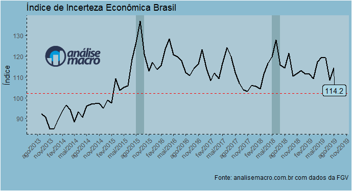
O índice registrou 114,2 pontos em agosto, acima da média representada pela linha vermelha tracejada. Aliás, diga-se, o índice vem se mantendo acima da média histórica desde 2015. Abaixo, colocamos um boxplot da série.
ggplot(data, aes(date, iie_br))+
geom_boxplot(fill='#8abbd0', color="black")+coord_flip()+
theme_classic()+xlab('')+ylab('')+
labs(title='Boxplot IIE-Br',
caption='Fonte: analisemacro.com.br')
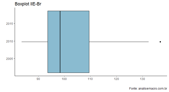
Como se pode ver no boxplot acima, o valor registrado em agosto está no último quartil. Em outras palavras, a incerteza permanece elevada no país.